After this tutorial, you’ll know “in your bones” how to deal with the weirder stuff, when it comes to time-dependent values.
It’s easy to find formulas to plug into to for simple cases, like a steady DC voltage or nice sine waves with known peak values but what happens when things aren’t so straightforward? Say you have a wind turbine, generating voltage with a varying frequency and changing peak values and you want to figure out the average power? What then?
Here I aim to give you an intuitive understanding of how to transform complex repeating waveforms (like AC voltages) into usable steady-state values to characterize results of interest (like average power). It gets into the actual why and how we calculate this stuff (without any calculus or heavy math–nothing beyond high school algebra), and by the end you should be able all the weird and various cases that life throws at you. It also lets you know how to get by without even knowing the peak or frequency values.
In these more arbitrary instances, you need to have a clear understanding of how we go about determining effective replacements for our complex varying values. Most resources either give you a formula for some specific case, out of the blue, and tell you “use this”. Or they drown you in equations and methods that you may have long forgotten by now. Here I offer–what I hope is–a complete explanation without any tough math but without going the rote memorization route, either. The goal is that, once you get through it, you’ll never have to refer to it again.
Ok, one thing: I lied. There is one little tidbit of calculus in here, but it’s something you probably do remember: integrating a function over a certain range is analogous to measuring the area “below” it, in that range. That’s it. With this notion in mind, we can figure out where the all formulas come from and apply our knowledge to deal with more interesting cases.
Throughout, the central example will be average power calculations based on instantaneous values of a varying voltage but we’ll cover other interesting cases (like torque) to show how general the approach is.
Dead-easy stuff: DC Power
Insta-refresher: for a simple DC circuit power is just
P = IV
or, equivalently using Ohm’s law,
P = I²R
or
P = V²/R
Whichever works best. In most cases, you have easier access to the values for voltage and resistance, so I’ll mostly stick to equations dealing with voltage here but the logic is the same in any case.
With a time-varying signal–where V and I are functions of time–the instantaneous power is
Pinst = I(t)V(t)
or
Pinst = V(t)²/R
But who cares about instantaneous power? What’s usually of interest is the average power delivered and, when you’ve got sinusoidal or other cyclical functions for V and I, things can get pretty messy.
Getting average power from cyclically varying voltages
If you’ve got a repeating sinewave-like signal, you can get by and figure out the average power by acting as if this varying value were in fact a simple DC voltage and use that in the DC formula from above. But to do this, you need to find some value that truly reflects what’s happening… What DC voltage that would be equivalent to that periodically varying value?
The canned answer, usually offered with only a summary explanation, is: use the Root-Mean-Squared (RMS) voltage, also known as the effective or effective heating value.
When you manage to convert your time-varying voltage to a this RMS value, you can act as if it were as a steady state, and the average power is just:
Pavg = Vrms²/R
For a clean and perfect sinusoidal voltage, it turns out the RMS voltage value is simply:
Vrms = Vpeak/√2 = 0.7071 * Vpeak
which is perfect when you know Vpeak and don’t care about how this works.
What happens if you don’t have a cleanly varying voltage, or if it’s not a perfect sine wave, or what if you don’t even know what the peak voltage is in reality?
You’ll find that you can also get this Vrms value by sampling the actual value of voltage at a number of points along the cycle and then use a little formula to figure it out, using those discreet samples. Online, you’ll find plenty of spots that teach you that, in the discreet domain, Vrms is just:
Vrms² = average of the squared values = ((V1² + V2² + … + Vn²)/n) for some n samples.
A quick test to verify that this makes any sense at all is to apply the formula to some DC voltage, V. This would then be
Vrms² = (((V² + V² + … + V²)/n)
Since the sum has n terms of V² this simplifies to
Vrms² = ((n(V²)/n)
The n’s cancel and we take the square root of both sides and you’re left with
Vrms = √(V²)= V
Just what you’d expect, as that would imply that
Pavg = V²/R = i.e. good ol’ P
and all is well.
Why we actually use RMS
Ok, that’s great. But why the hell are we doing this? The short of it that, whether we’re plugging in voltage or current, the power physically depends on some squared value.
So if we’re going to be replacing the time-dependent function by some constant average value, then that value needs to give an accurate reflection of the world when squared — i.e. f(t) must be approximated to some constant C such that when C is squared (C*C) it has the same effect, on average, as f(t)*f(t). So what we’re looking for is the average of the squared function and, when all is nice and simple, you can just use the method above.
For our power as a function of voltage, what we’re really doing here is taking the time-dependent V(t) ~ sin(t) and squaring it, which looks like:
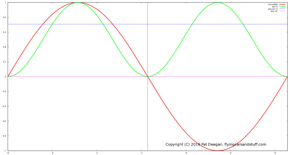
In red is the actual value of the voltage at any given point in time. Once you square that value you’re basically looking at the green curve, instead, which is always positive–a nice feature that avoids worrying about the average value being 0 over a full cycle–and will give us something to work with… ok, now we’re getting somewhere.
What is the average value of this V(t)² curve? You can do some nice calculus to figure it out (you’ll find that integrating to get the area under the green curve from 0 to π is π/2 and go from there) but the short of it is that this green wave is symmetric about it’s mid-value and its mean (average) turns out to be 1/2.
So the average of the V(t)² is 0.5… but what we wanted at the beginning up there was actually the average effective voltage, not the average squared, so we need to get rid of this using a square root… and √(1/2) just happens to be: 0.7071! And that’s where the magic value comes from.
These calculations were done with a sine wave with an amplitude (peak) of 1 but it all scales linearly with amplitude, which is why the formula for a sine’s Vrms is:
Vrms = Vpeak * 1/√2 = Vpeak/√2
Practically speaking it doesn’t actually matter exactly how many voltage level readings you take, with these two caveats:
- you should have many points (samples) within a given period, to get an accurate representation of the curve (see Nyquist etc); and
- your samples should be taken over a whole number of half cycles to get the true RMS value
In essence, if you had a voltage as depicted here going from -1 to +1V, the value of your total sum of squares will go up by (on average) 0.5 for every sample you take, but then you’ll also be dividing by a larger n which would bring the result back down to what it should be.
To illustrate, say you’re sampling n times per half-cycle, and you wind up sampling over 2 full periods (i.e. 4 half-cycles). For simplicity, lets assume that the first readings you make in each half-cycle all come out to the exact same value, V1, the second all come back as the same V2, and so on. You’ll end up with:
- a sum of voltages-squared for each half cycle: (V1² + V2² + … + Vn²); and
- a total 4n samples
So
Vrms = √((V1² + V2² + … + Vn²) + (V1² + V2² + … + Vn²) + (V1² + V2² + … + Vn²) + (V1² + V2² + … + Vn²) /4n)
= √(4(V1² + V2² + … + Vn²)/4n)
= √((V1² + V2² + … + Vn²)/n)
which is brings us back to where we started. Cool.
Sampling Interval
So we know that we can figure out Vrms even without out knowing Vpeak but the above still assumes you can stop your sampling after 1 or more complete half-cycles–meaning you have to know the frequency of the varying voltage and make sure to only add values over some whole number of (half) cycles.
What if you don’t know the actual period? If you find yourself measuring the output of a wind turbine or are using running hamsters to rotate your generator or something else where you can’t know the frequency in advance, what should you do?
To rephrase, the question is: what happens when you’re taking samples over some non-integer number of half-cycles?
For some extra samples, k, forming an incomplete half cycle (so k<n, where n is the number of samples taken in a given period), some error will be introduced into your calculated Vrms. In the case of a steady DC voltage, this would not be the case, as even after we’ve added the additional sum components:
V1² + V2² + … + Vk²
We’d end up with n+k total samples and the RMS voltage would be:
Vrms² = (V1² + V2² + … + Vn²) + (Va² + Vb² + … + Vk²)/(n+k)
but since it’s DC all the samples are identical and can be replaced by value V:
Vrms² = (nV² + kV² / (n + k)
= (n+k)V²/(n+k)
= V²
This is true because, no matter where it’s taken in the cycle, a sample always adds the same amount to the sum: in other words there is a strictly linear relationship between the number of samples and the sum.
But in the case of a sine wave the relationship between number of samples and running total is non-linear, so the sum of the squared samples isn’t directly proportional to the number of samples taken.
With a time varying cyclical signal, the RMS voltage is actually defined as:
Vrms = √( (1/T) * ∫SOME UGLY INTEGRAL OF A FUNCTION V(t)² TAKEN OVER THE PERIOD )
Recalling that tidbit of calculus I mentioned right at the start, taking “SOME UGLY INTEGRAL…” over some interval is the same as figuring out the area under the function in that interval. What we’re doing with our samples is basically approximating this by summing a bunch of tiny rectangles with a “height” related to our sample value and a width of some small time interval dt.
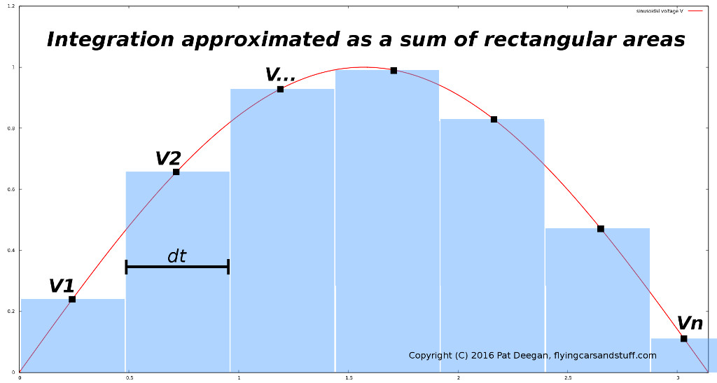
When you add all these together, you get a good approximation of the the area under the curve (well… “good approximation” as long as dt is small compared to the period T):
Area = ∑(Vi*dt) = (V1²*dt + V2²*dt + … Vn²*dt) = (V1² + V2² + … + Vn²) * dt
So now, instead of dealing with that unwieldy integral, we have the RMS voltage defined as
Vrms = √( (1/T) * Area)
= √( (1/T) * (V1² + V2² + … + Vn²) * dt)
This is still ugly though, because our Vrms seems to depend on the period of the signal, T, and also on whatever time slice we’ve selected, dt.
But there’s good news… whatever we choose for our interval between samples, dt, we know one thing: the number of samples over a complete period is going to be
n = (T/dt) samples
Rearranging, we can define T in terms of n and dt:
T = n*dt
If you plug this representation of T in our definition for Vrms, you get
Vrms² = (1/T) * Area
= (1/(n * dt)) * Area
= (1/(n * dt)) * (V1² + V2² + … + Vn²) * dt
= (V1² + V2² + … + Vn²) * dt / (n * dt)
= (V1² + V2² + … + Vn²)/ n
Well, that looks pretty familiar! This is how we know that the famous technique for discreet Vrms approximation is actually usable and true to reality.
Now we can determine a few more things. First off, if you sample multiple periods rather than just one, it doesn’t actually matter. Say you tabulate values for x periods rather than just the one, then call:
Areanew = Total area tabulated = Area * x
because you’re adding the area under the function x times. However, you’ve been integrating over a new “period” Tnew that is x times longer than T:
Tnew = x * T
Plug these into the formula for Vrms and the x‘s cancel out:
Vrms² = ( (1/Tnew) * Areanew )
= ( (1/x*T) * x * Area)
= ( (1/T) * Area )
so we’re back in business as before.
Dangling samples: sampling over arbitrary time intervals
What if you sample for, say, a full period plus some extra fraction of a period (e.g. some time less than a full half cycle). Doing this obviously has two effects:
- it increases the total area (the value of the integration); and
- it increases the number of samples
Does the amount of time the sampling occurs actually matter?
Unlike for a steady DC voltage, with time-varying signals the answer is yes it does matter. This is because when you add 1 sample, you increase the number of samples by 1 but you don’t necessarily increase the total area by exactly (Area/n), since the value function is non-linear.
Check this awesome graph out:
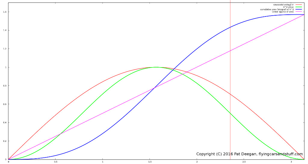
Here you can see the voltage as a function of time (a beautiful sine wave, here), over one half period, in red. The green line represents the squared, V², value as a function of time — that’s the thing we’re interested in integrating.
Along with these two functions are:
- the real cumulative count of the area under the V² curve (value of the integral) at any corresponding point in time (blue); and
- the cumulative value of the integral, if it was actually linearly dependent on the number of samples taken (i.e. if the voltage function were actually steady-state, a constant DC voltage)
If you plug in your samples values for an incomplete cycle and use them to calculate Vrms, you’re acting as if each slice contains the same amount of area. This is incorrect and introduces error.
The distance between the blue curve (integral) and the approximated linear curve at any given time is the amount of error you’re introducing if you stop sampling at that moment and calculate your RMS value based on what you have so far. You can see there’s no error when you have 0 dangling samples (because you have a complete number of half-cycles) and at the half-way point because of the waveform’s symmetry in this case. Stop at any other point to calculate Vrms and you’ll have some error.
When assuming the sum grows linearly, you basically overstate the importance (the relative contribution) of samples early on (the values are small, compared to the average contribution, so your estimated RMS will be too small) and, past the midway point, your linear guess is out of whack in the other direction (because future contributions will be getting small quickly, as you can see the blue curve growth slow to a crawl).
This error in the weight to give the contribution from a partially sampled (half) cycle can go up to ~25% in the worst cases (where you’ve sampled 1/4 or 3/4 of the half-period, have a look at the difference between the approximation and the true value at the time indicated by the vertical red line).
What we’d like to know is the actual effect on our calculation for Vrms: how bad is it? Going with the linear approximation, by simply adding our sampled V² values areas and incrementing the sample count, here’s what happens in the worst case.
Say we have
n = samples/cycle
k = number of dangling samples from incomplete cycle
As mentioned, taking a straight average using dangling samples is equivalent to assuming the contributions over a cycle grow the area linearly (following the linear approx curve) and we know that at most points this guess is inaccurate.
To figure out just how inaccurate, lets say our session includes one full cycle plus a number of dangling samples k–lets check our worst case, at the 3/4 mark. In this case, the linear approximation of the integration for this cycle will be off by 25% of what is would be after truly integrating up to that point.
Now define:
Area = actual area under curve for a full cycle,
Areak = k samples area contribution = (3/4) (Area + 25% of Area) = (3/4) ( 5/4 Area) = (15/16) Area
AreaTot = total area determined by our algorithm = Area + Areak = Area + (15/16)Area
T = period over one true cycle,
Ttot = total pseudo-period for this sampling session = T + (3/4)T = (7/4)T
Our calculated Vrms, with contributions from the full cycle sampled plus the k dangling samples, becomes:
Vrms = √((1/Ttot) * AreaTot)
= √(4/7T * (Area + (15/16)Area))
= √(4/7T * (31/16)Area )
= √((31/28) (1/T) * Area)
So, compared to what it should be, we’re actually reporting √(31/28) of the true value… so off by about 5%. pff… not so bad.
More generally, if we’d sampled a number of full cycles before actually collecting those dangling values, say x cycles, we’d have instead:
Ttot = xT + (3/4)T = ((4x+3)/4)T
AreaTot = xArea + (15/16) Area = ((16x+15)/16) Area
And so
Vrms = √((1/Ttot) * AreaTot)
= √(4/(4x+3)T * ((16x+15)/16) Area)
= √( ((16x + 15)/(16x + 12)) * Area/T)
As you can see, as x gets bigger and bigger, the small constant 12 and 15 terms become more negligible and the error for our estimate goes down towards 0. For example, with 10 full cycles and 3/4 cycle of dangling samples, the reported value will be:
√((160+15)/(160+12)) = √(175/172)
so 1.009 times the value it should be (or 0.9% too large), in this worst-case scenario.
Other types of waveforms: putting understanding to work
Now that we have a good grasp on what we’re doing and why, we can see how to confront some other typical problems you might encounter.
Most of the formulas around, like
Vrms = 0.7071 * Vpeak
only apply to clean sinusoidal functions. But, as we’ve seen, the discretized method of summing a stream of regularly spaced samples is equivalent to calculating the integral and works for any repeating waveform.
An easy example is the same sine-wave varying voltage, but half rectified so that only the positive voltage swings are delivered to your circuit.
If n is the number of samples taken in half of a cycle, then our total number of samples in a full cycle will be 2n and our RMS voltage will be:
Vrms² = (V1² + V2² + … + Vn²) + ( 0 + 0 + … + 0)/ 2n
= (1/2) ((V1² + V2² + … + Vn²))/n
so we come to the conclusion that dropping half the squared values bring our Vrms² value down by half which makes a lot of sense.
Since we know
(V1² + V2² + … + Vn²))/n
is our Vrms² for a unrectified (or fully rectified) signal, we can say
Vrms-half-rectified² = (Vrms²)/2
If you use the simple Vpeak formula in place of Vrms, then
Vrms-half-rectified² = (1/2)(Vpeak²/2) = Vpeak²/4
Vrms-half-rectified = Vpeak/2
which matches what you find anywhere there’s a list of formulas. Hm, guess we no longer need no blasted formula lists. Good.
Example: Torque and rotational power
What if we’re looking at calculating other kinds of power? Say you’ve got some way of measuring instantaneous torque and would like to calculate the average power delivered.
Power, in the case of a force rotating something, is
Power = 2π * torque * rotations per second
Now if the torque is constant this is all straight-forward, as in the case of the DC circuit power calculations above.
But what if the torque is, say, coming from the force applied to a bicycle pedal? You know how long the pedal arm is and you have some sensor on the pedal to measure force, so you can get instantaneous values of torque at any moment, represented by some voltage:
torque(t) ~ v(t) ~ some periodic function of Bob’s foot on the pedal
The force on the pedal will vary with time, and in this case will most likely look like a half-rectified sine wave if Bob is an average bicycle user. We’ve covered that wave form, above, but do our previous methods apply?
Actually, since the power is a function of torque
Pavg ~ torque(t) ~ V(t)
and not of torque squared, the answer is: not quite.
Here, we will want to use a estimated constant value of torque that represents reality when used *as-is*–it is not used squared. So is any of our work so far useful in this case? Yes, because the exact same approach applies. The differences are mainly that:
- we won’t be taking the average of the squares, but the average of the (magnitude) of the voltages (~torque) themselves; and
- the error from dangling samples will actually count more
Here’s a graph similar to that above, showing the sine-varying measured value, the real value of integration over 0 to any point and the linear estimation.

You can see that after one full cycle, the area below a sinewave (with a Vpeak of 1) is exactly 2. Since one cycle of a simple sine curve has a period of π, the average V is
Vavg = Area / period = 2/π
Similarly to last time, this result was found for an amplitude (a peak) of 1 but will scale linearly so you can just multiply it for sine functions with greater amplitude. So this is where the
Aavg = Apeak *2/π = Apeak * 0.637
formula you’ll encounter comes from.
Though the amount of error between the actual integral at any point and the linear estimation is reasonably similar, since we won’t be taking the square root of the result, it’s actual effect will be greater than in the above example having dangling samples from the start of a cycle to the three-quarter mark.
Still, if we’re sampling over a number of cycles before adding in the dangling entries, then the error still reduces quickly. For instance taking in 5 full periods worth of samples plus an addition 3/4 cycle of danglers, and assuming the same 25% error as above, you wind up being off by about 3%, and after 10 cycles you’re below 2%–and this is the worst case! Not too shabby.
On the down side, if your samples go negative you need to ensure you either tally your average only during the positive swing or you do so using only the magnitudes (i.e. the absolute values) otherwise all your full cycles will just cancel out and you’ll get an average of 0 (if you happen to be sampling over complete cycles, if not your average would be badly messed up… so yeah, use magnitudes).
An even greater downside is that, in the case of power from applied torque, you really do need to know the period of the cycles in order to get a value. But this a problem for which a simple solution was already discussed.
The moral of the story for average power from torque is thus that we can use our discreet method to do it, but:
- we’ll need to take the average of the magnitudes of torque (not the squares),
Vavg = (||V1|| + ||V2|| + … + ||Vn||)/n; - the impact of dangling samples will be greater, unless we ensure we’re sampling over some decent number of cycles (e.g. 5 or 10);
- we’ll need some manner of converting Vavg to average torque; and
- we’ll need to figure out the period of the input voltage function to actually calculate the Power = 2π * Tavg * rotations per second
Ohm’s law for varying voltages
This thinking applies to any case where you’re trying to find the DC equivalent of a function that depends linearly on a time-dependent cyclical value, for instance the average current through a LED.
I(t) = V(t)/R
so
Iavg = Vavg/R
With Vavg being determined in the same way as our torque above. This should work nicely for anything Ohm-ish.
Conclusion
At this point we know some handy formulas for simple cases but, more importantly, have a good idea of how to do power and other types of calculations when all we have access to are instantaneous samples of some cyclical value.
The main lesson is therefore that, unless we already know the exact frequency of our signal and can perform our sampling over a single period, then it’s better to ensure we do so over at least a few cycles in order to minimize the error in our discretized integration.
Of course, if the frequency and/or amplitude of your signal is varying with time, then sampling over too many periods will lead to another kind of error, so the trick is to find the right balance between reducing the influence of the dangling (extra) samples and only sampling during a total period where the repeating pattern will be roughly constant.
Hopefully, I’ve been able to provide a deeper understanding of how you can deal with these sorts of cases and of where all the formulas you’ll encounter in this domain come from. The approaches described should help with any calculation involving reducing some complex cyclical waveform to a usable and realistic average value.
Have fun!