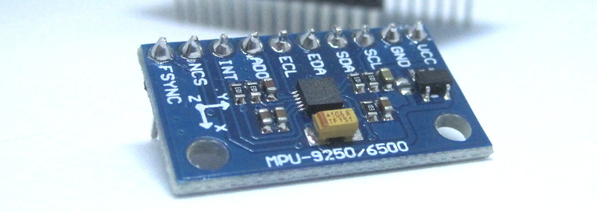
Though I’d used the Razor 9DoF and a few other IMUs, it’d been a few years since I got to play with an AHRS.  Recently, I got a request to tweak a system using the MPU-9250, a nine-axis (gyro, accelerometer and compass) MEMS device, to see how nicely we could get it to play.

I didn’t have the target hardware  (a custom system with the motion tracking, as well as GPS and other peripherals) on hand, but I did have an MPU9250 breakout.  So I agreed to take a look at how much performance and, most importantly, how much reliability (i.e. low drift) I could squeeze out of the device on a first pass.

Spoiler: I’d say it works pretty well.  This video shows a quick look at the results, which I’ll detail in the following.  Note that I didn’t actually care that the axes match-up, and it looks like the yaw’s sign was inversed… anyway, check it out:

Though I could have started with the existing codebase, it was a tangle of spaghetti dealing with all that extra hardware/sleep modes and setup to run on a Simblee (which I don’t have around, anyway), so I opted to start fresh and determine what the theoretical best case would be before merging into the system.  So the first step was to get talking with the ‘9250.

Talking to the MPU-9250

There are numerous libraries available online for this, but I was restricted to something that would be able to communicate over SPI because of the existing boards on the client side.  The MPU-9250 can use either SPI or I2C, but most of the libs seem to focus on I2C–nice, as it takes fewer lines, but slower, and not an option here in any case.

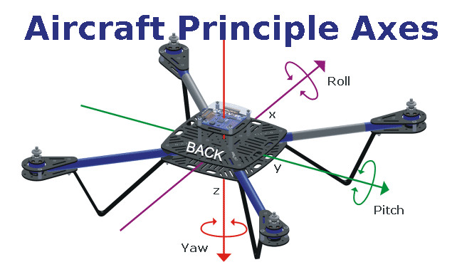
I did find a nice library by Bolder Flight Systems that actually supports both modes.  It was good enough to give me access to the raw data, but I needed to transform these 9 instantaneous values into actual heading and attitude–i.e. aircraft principle axes (roll, pitch and yaw).  Enter the magic of the quaternion representation filter presented by Sebastian Madgwick in 2010.

One of the great things about the Madgwick algorithm–other than the fact that it works pretty smashingly–is that there are a bunch of open source implementations available.

So I augmented the borderflight library to support the filter and auto-update it on reads of the sensor (currently available in this branch of my fork of the project, though perhaps pulled into the main tree by the time you read this).  I’ve included an AHRS example in the release, but the gist of the HOWTO is this:

1. Create IMU and a Madgwick filter objects;
2. Do a little setup work;
3. Regularly read the sensors, passing the IMU object the filter to update; and
4. Query the filter’s getRoll(), getPitch() and getYaw() whenever you want to know what you’re looking at.

Most of the “knobs” you can tweak have to do with the frequency of the updates and the low pass filter set on the MPU9250, explored a bit below.

Configuration

Though the library provides for calibration–it auto-calibrates the gyro at start-up and can let you discover and set calibration values for the accel and mag sensors–and it is a good idea to do so for each MPU and installation, that’s covered in the lib documentation… here I’ll focus on the settings related to the AHRS itself.

Other than actual sensor calibration, getting accurate/low drift results depends on two main factors:

1. crunching lots of (sensible) data; and
2. giving the Madgwick filter an accurate sense of time.

Obviously, if you want roll/pitch/yaw to reflect reality, you can’t just sample the accel/gyro/mag once every couple of seconds… you want to sample early, sample often.  How you arrange for this will be implementation specific, but you want regular and frequent updates for the filter to consider.  The AHRS example uses a simple delay in the main loop, but in real life you’ll probably have more to do so using the data ready interrupt is likely a good option.

Related to this is the precision and value of the data… the tweaks here involve using the lowest ranges for the sensors that won’t clip the values and Digital Low Pass Filter (DLPF) bandwidth and data output rates.  These must be selected wisely, and there’s a good section in the library’s README about those.

Once you’ve figured all that out and put appropriate calls in your setup routine, the final element is the Madgwick “sense of time”.  In this case, the algorithm wants to be told how often the updates you’re sending it (through the call to readSensor(FILTER)) are actually happening.

This is set by passing the frequency as a parameter to the filter’s begin(), i.e.

   MyMadFilter.begin(FREQUENCY);

Let’s say you’ve determined that you’ll be reading the MPU (and hence updating the filter) every 5ms.  In this case, you’d be updating at 200Hz, so

   MyMadFilter.begin(200);

In my testing, I was using a delay(5) call so in theory 200Hz… but there’s overhead in between the main loop calls, during the data processing, etc.  So, to get the best performance, this number was reduced slightly (e.g. about 180Hz on a ATMega328 system running at 8MHz).

Visualisation

Though checking the numbers output through the UART told me that things seemed to be working quite nicely, I wanted something more visual that I could gauge in more direct terms.

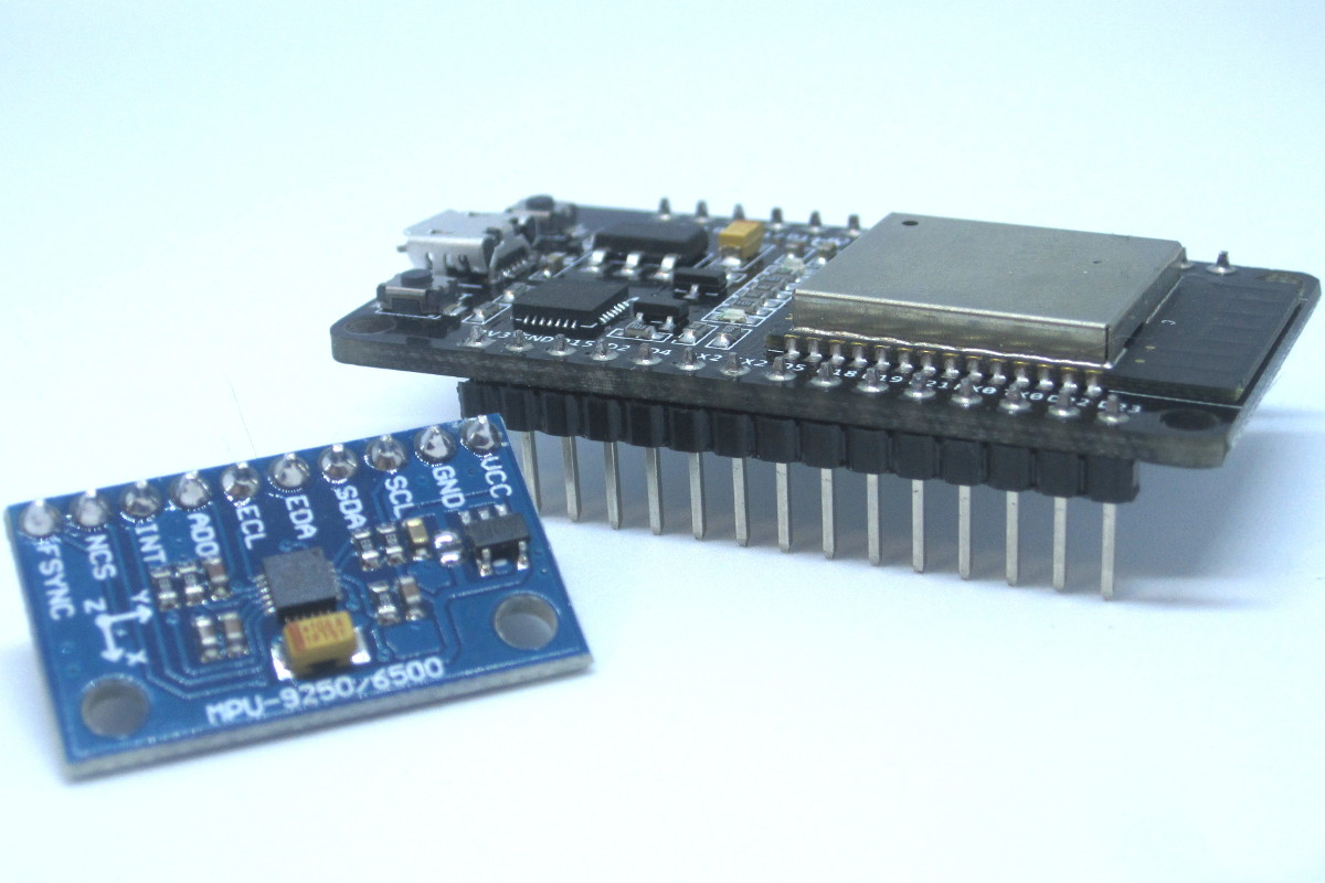
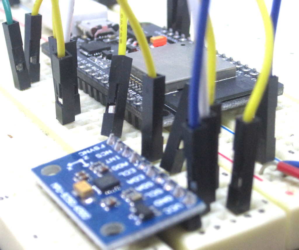To do so, I replace the mega328 driver by an ESP32 in order to get access to the oh-so-sweet bluetooth low energy available through the device.  I wired it all up on a breadboard and confirmed that the AHRS example would run.  Once that was confirmed to be running well, I set up a small program to provide a BLE service with a characteristic that would output notifications.

These notifications are just the twelve bytes that comprise a bundle of the three float values for roll, pitch and yaw.

When the ESP32 was accepting connections and spitting out the values, I whipped up a small Android app to connect to the ESP32, and subscribe to the notifications.  Since this is a cordova app (therefore based on simple HTML/JS, while having access to underlying hardware like bluetooth), it  also gave me a chance to try out three.js, an extremely cool lightweight library to give you the power of WebGL acceleration.

So I setup a little scene, camera and basic crate to act as a proxy for my breadboarded IMU mess-o-wires.  The result is the video at the top of the page, which shows the system providing pretty decent results.

Final Notes

One final thing to note is that there’s a period between startup and the point at which the Madgwick filter has settled down to what it believes is the chips actual orientation.  I think this has to do with the initial values for the quaternions.  It seems that, though for the most part a small timeslice (i.e. high sampling rate) is a good thing, the smaller this timeslice the longer the settling time on startup.  So that’s one more thing to consider in your tradeoffs, but assuming the system is on for relatively long periods, it shouldn’t be a big deal either way.

So that’s it for this presentation of my little experiment.  Hopefully, you can use this info and the library to make your own cool direction-aware projects.  Have fun.